NLP Course - Neural Language Models Notebook
Introduction to Neural Language Models
A neural language model (NLM) is a machine learning model used in natural language processing (NLP) to predict the probability of a sequence of words or the next word in a sequence. Unlike traditional statistical models like n-grams, NLMs use neural networks to learn complex patterns in text, capturing both semantic (meaning) and syntactic (grammar) relationships.
Key Concepts
- Purpose: Predicts P(wₙ | w₁, ..., wₙ₋₁), the probability of the next word given the previous words.
- Advantages: Can capture long-range dependencies, understand word meanings, and scale with large datasets.
- Applications: Used in text generation, speech recognition, machine translation, and autocomplete systems.
How Neural Language Models Work
Neural language models take a sequence of words, process them through a neural network, and output probabilities for the next word. For someone new to this, think of it like a smart system that learns from examples to guess the next word in a sentence. Here’s how it works step-by-step:
Step-by-Step Process
- Input Text: Start with a sequence of words, like "The cat is".
- Word Embeddings: Convert each word into a numerical vector that captures its meaning (e.g., "cat" might become [0.1, -0.3, 0.5]).
- Neural Network Layers: Pass these vectors through layers (like fully connected layers) to learn patterns in the sequence.
- Output Layer: Use a softmax function to produce a probability for each possible next word in the vocabulary.
- Training: Adjust the model’s parameters (weights) to make better predictions by minimizing errors using a loss function, like cross-entropy.
The model learns by seeing many sentences and tweaking its internal settings to improve its guesses.
Word Embeddings
Neural networks can’t process words directly because they’re text, not numbers. Word embeddings solve this by turning words into dense vectors (lists of numbers) that represent their meaning in a numerical space. Words with similar meanings (like "king" and "queen") have similar vectors.
How Embeddings Work
- Representation: Each word gets a vector of fixed size (e.g., 300 numbers). For example, "cat" might be [0.1, -0.3, 0.5].
- Learning: Embeddings are learned during training (e.g., using Word2Vec or GloVe) or loaded from pre-trained models and fine-tuned.
- Example: For the input "The cat", embeddings might look like: The → [0.2, -0.1, 0.4], cat → [0.1, -0.3, 0.5].
Example Code
Softmax Function
The softmax function is used in the output layer of a neural language model to turn raw scores (called logits) into probabilities for each word in the vocabulary. These probabilities sum to 1 and show how likely each word is to be the next word.
Intuitive Explanation
Imagine you have scores for possible next words: 2.5 for "jumps", 1.0 for "sleeps", and -0.5 for "runs". The softmax function makes these scores positive and scales them so they add up to 1. For example, it might give 0.7 for "jumps", 0.2 for "sleeps", and 0.1 for "runs". It boosts higher scores while still giving small probabilities to less likely words.
Mathematical Formulation
For a vector of logits z = [z₁, z₂, ..., zₙ], the softmax function computes the probability for the i-th word as:
Here, e^{zᵢ} is the exponential of the i-th logit, making all values positive. The denominator sums the exponentials of all logits to normalize the probabilities.
Key Points
- Exponentiation: The exponential function e^x ensures all outputs are positive and amplifies differences between scores.
- Normalization: Dividing by the sum ensures the probabilities add up to 1.
- Challenges: For large vocabularies (e.g., 100,000 words), computing softmax is slow, so techniques like sampled softmax or hierarchical softmax are used.
Example Code
Activation Functions
Activation functions add non-linearity to neural networks, allowing them to learn complex patterns. Without them, a neural network would just be a series of linear transformations, which can’t model things like the relationships between words in a sentence. They decide whether a neuron should "fire" or pass information forward.
Common Activation Functions
- Sigmoid: Maps inputs to [0, 1], often used for binary decisions.
σ(x) = 1 / (1 + e^{-x})
- Pros: Outputs can be interpreted as probabilities.
- Cons: Causes vanishing gradients (gradients become very small) for large inputs, and it’s not zero-centered, which can slow learning.
- ReLU (Rectified Linear Unit): Outputs the input if positive, otherwise 0.
ReLU(x) = max(0, x)
- Pros: Fast to compute, avoids vanishing gradients for positive inputs.
- Cons: "Dying ReLU" problem, where neurons stuck at 0 stop learning.
- Tanh (Hyperbolic Tangent): Maps inputs to [-1, 1], centered at 0.
tanh(x) = (e^x - e^{-x}) / (e^x + e^{-x})
- Pros: Zero-centered, which helps gradients flow better during training.
- Cons: Still suffers from vanishing gradients for very large inputs.
- Softmax: Used in the output layer for multi-class problems like predicting the next word (described above).
Example Code
Why Tanh is Widely Used
The hyperbolic tangent (tanh) activation function is commonly used in neural language models, especially in early models, for several reasons:
- Zero-Centered Output: Tanh outputs range from -1 to 1, with a mean of 0. This helps gradients flow better during backpropagation compared to sigmoid, which outputs 0 to 1 and can bias updates.
- Non-Linearity: Tanh allows the model to learn complex patterns, like the relationships between words in a sentence.
- Better Gradient Behavior: Compared to sigmoid, tanh has stronger gradients near the origin, aiding optimization, though it still suffers from vanishing gradients for extreme inputs.
- NLP Suitability: In word embeddings and hidden layers, tanh captures both positive and negative relationships (e.g., synonyms vs. antonyms), which aligns with linguistic structures.
While modern models often use ReLU or its variants for faster training, tanh remains popular in recurrent neural networks (RNNs) and early NLP models due to its balanced properties.
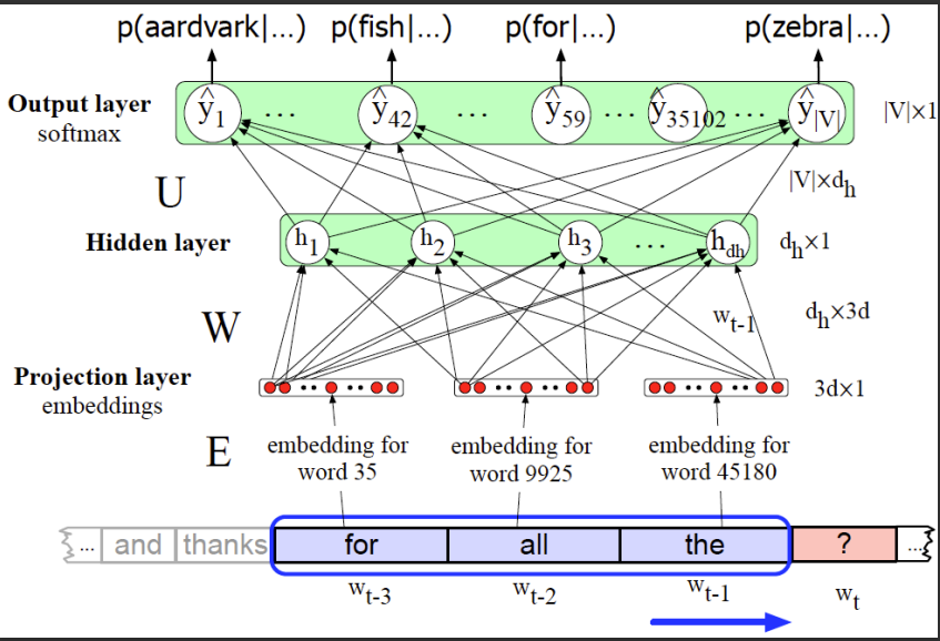
Fixed Window Problem
Basic neural language models often use a fixed-size context window (e.g., the previous n words) to predict the next word. This approach has limitations:
- Limited Context: A fixed window (e.g., 5 words) can’t capture long-range dependencies, like relationships across sentences or paragraphs.
- Input Size: The model expects a fixed number of input words, requiring padding or truncation for shorter or longer sequences.
- Scalability: Increasing the window size increases computational cost and model complexity significantly.
These limitations make fixed-window models less effective for long sequences. Recurrent Neural Networks (RNNs), which maintain a hidden state to remember past information, address this issue by processing sequences of arbitrary length. We’ll cover RNNs in the next notebook.
Practical Example
Let’s implement a simple neural language model using a feedforward neural network with word embeddings, a hidden layer with tanh activation, and a softmax output layer. The model predicts the next word given a context of two words (bigram). We define a small vocabulary and simulated data, initialize embeddings and weights, and perform a forward pass to compute probabilities and loss. This is a simplified example; real models would include a full training loop and optimization.